***** MONTCARL *****

Monte-Carlo simulations of light transport in transparent or turbid media, like tissue,

with Scattering, Absorption, Fluorescence, Raman, Laser-Doppler and Photo-acoustics,

with layers and objects, like spheres, tubes, cones, mirrors, lenses, pupils, diaphragms.

back to home screen

Keywords: Download Programs: Scroll down	Light scattering and transport, with: · Events: scattering, absorption, reflection, refraction, transmission, with cross sections and attenuation coefficients, · Scattering functions: Mie, Dipolar, Rayleigh, Gans, Henyey-Greenstein, Gegenbauer, or Isotropic, Fournier-Forand, with fluorescence and Raman-scattering, · Layers and objects: tubes, spheres, blocks, toroids, cones, mirrors, lenses… · Ray tracing and Imaging through transparent and turbid lenses, pupils, diaphragms, mirrors…. · Extra’s: frequency modulation, Doppler frequency, Laser-Doppler flowmetry, skin tissue, path tracking, flight tracking, Photo-Acoustic signal production. · Table of suggested optical properties in tissue.
MOVIES	View MOVIES: 1. Full DESCRIPTION OF THE PROGRAM (incl. photon transport process): video : movie 2. LIGHT SCATTERING BY PARTICLES, theoretical models and derivations: pdf-file I. Light scattering theories and models: video: part I II. Derivations of dipolar and general scattering expressions: video: part II 3. TRANSPORT PROCESS OF PHOTONS in the medium: video: MP4-file 4. PHOTO-ACOUSTIC RESPONSE simulation using MONTCARL: video: movie
General objectives:	· · The program calculates Monte-Carlo simulations of LIGHT TRANSPORT IN TRANSPARENT OR TURBID MEDIA, WITH SCATTERING and/or ABSORPTION · optional: followed by FLUORESCENCE or RAMAN-scattering, or PHOTOACOUSTICS in turbid media, like tissue. · The SAMPLE may consist of a single or more LAYERS, each with its own absorption and scattering data, in the form of concentrations of scattering particles embedded in a medium. In order to register DOPPLER spectra, to each type of scattering particle a certain velocity vector can be associated. In each layer a number of separately defined structures (called "OBJECTS": with rectangular, cylindrical, spherical or conical shape) may be present, with similar characteristics as the layers. Option: spheres may be randomly distributed in a layer. With those objects e.g. blood vessels can be mimicked. Also transparent and turbid lenses and pupils /diaphragms…. · Also an oblique mirror plane can be inserted. Furthermore, the layers may be subdivided into sublayers (depth pixels, see below). · There are more options: internal light sources and external beams, internal and external detection, plots of distributions of various variables (photon positions, path length distributions, photon tracking, layer+object structure plots, frequency modulation by Fourier transformations, angular distributions, photo-acoustic response plots, ray tracking in lenses systems, ….
DOWNLOADS	· IMPORTANT: Remove old versions of Montcarl.exe first, to avoid possible interference !! · Demo or full version (your first download): Download montcarl.zzz here to a new or suitable folder. After download: (1) change *.zzz -> *.zip, (2) unzip *.zip into that folder, then (3) read “READ ME FIRST” and (4) rename MC_Install.fff to *.exe and run *.exe-file. MC_Install will create and install all necessary folders and files. · Updates: Download montcarl-update.zzz from here to your MONTCARL\PROG-folder; After download: (1) change *.zzz -> *.zip; (2) unzip *.zip into that folder; (3) change *.fff -> *.exe and (4) run *.exe-file. This download may also contain updated versions of HELP-files (*.pdf).
More information:	· Description of the program options · The physical mathematics behind the calculations · See also: List of publications
Options:	· Download the demo or full version of the program and work for yourself. · Let us do the simulations for you (first try-out free; contact us); this will save you a lot of work and time!

Examples of screens in the program:

All screen outputs with results also have print and file output in table format, compatible with Excel-like programs.

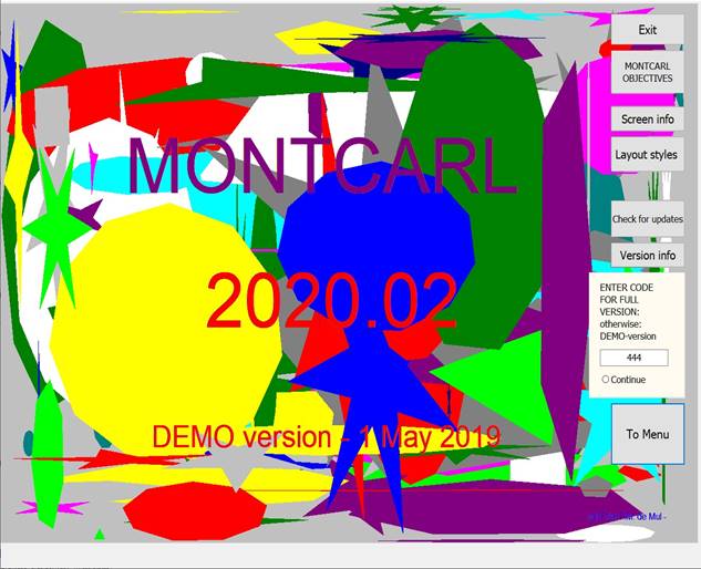
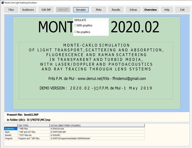
↓ Fig. 1. Begin screen of the program (choice of screen size and color)	↓ Fig. 2. Menu screen (with Tabs)
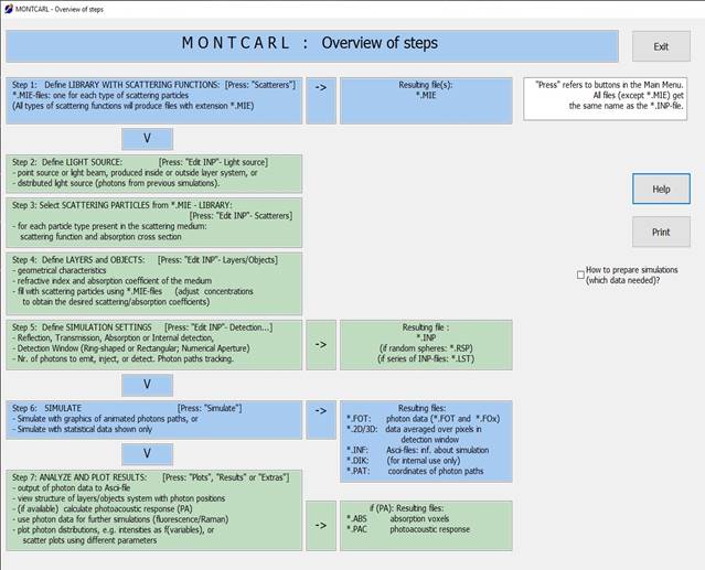
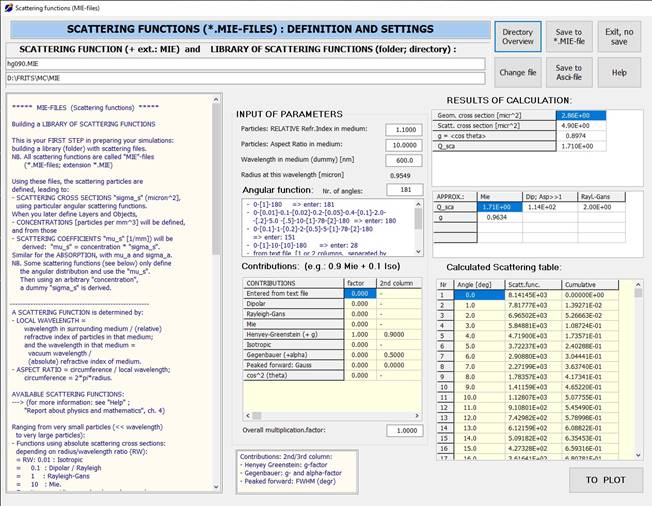
↓ Fig. 3. Overview about how to input settings and to run simulations	↓ Fig. 4. Creation of scattering functions (called: *.MIE-files)
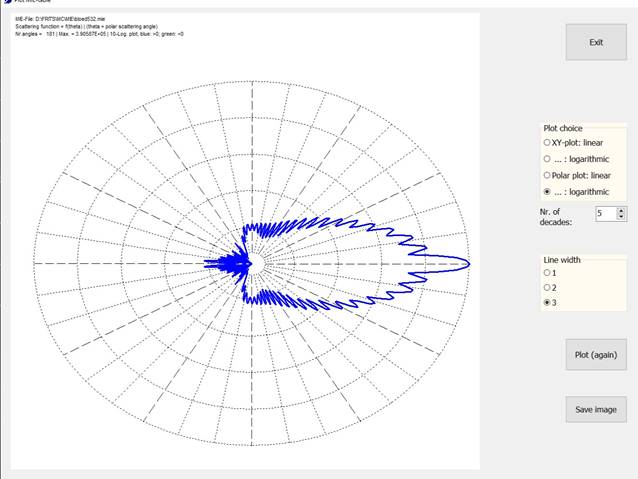
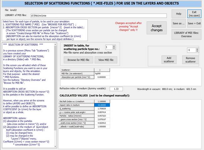
↓ Fig.5. A scattering pattern (combination: Mie + Henyey-Greenstein-functions)	↓ Fig.6. Selection of scattering functions for use in layers and objects
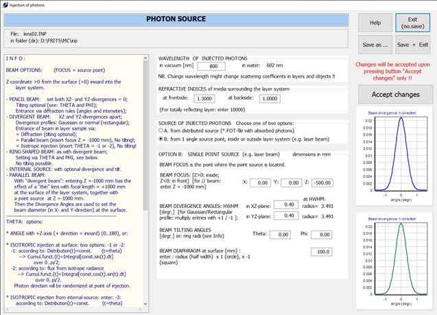
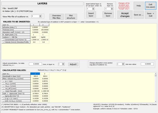
↓ Fig.7. Input of data for the light source (e.g. laser data)	↓ Fig. 8. Input of data for layers (more than 1 layer possible)
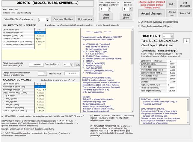
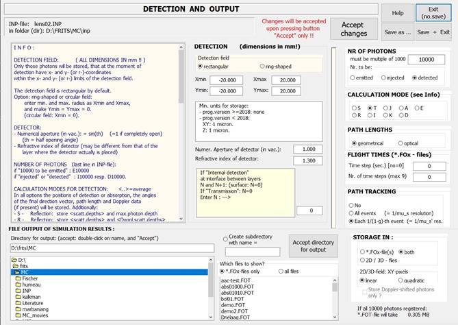
↓ Fig. 9. Input of data for objects (spheres, tubes, mirrors, cones, blocks…)	↓ Fig. 10. Detection, calculation mode, flight and path tracking and output
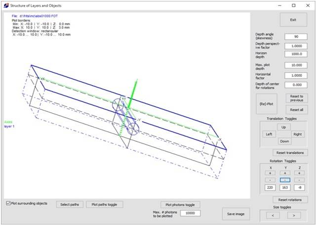
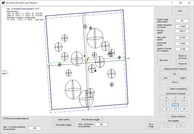
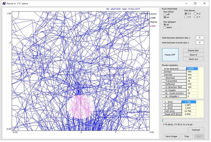
↓ Fig. 11. Structure of the layer system with 1 layer and 1 tube in Y-direction	↓ Fig. 12. Simulation of the structure of Fig. 11. View // Y-axis (XZ-plane)
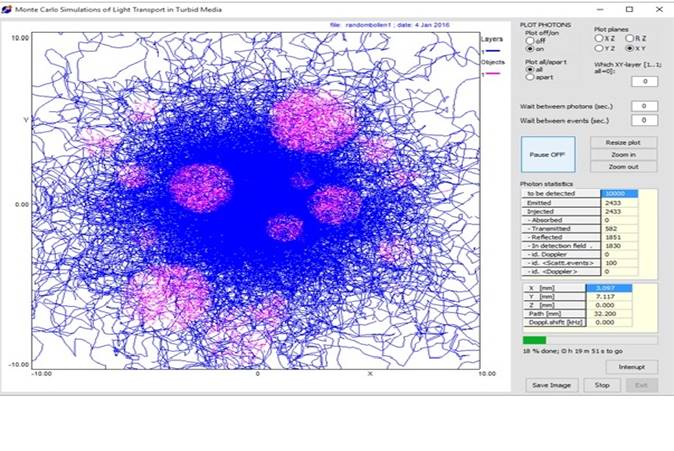
↓ Fig. 13. Structure of a single layer with random spheres	↓ Fig.14. Simulation of the structure of Fig. 13. View // Z-axis (XY-plane)
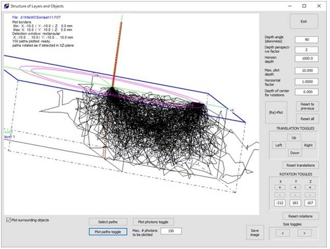
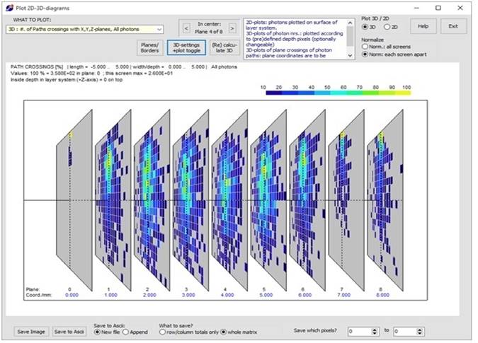
↓ Fig. 15. Path tracking for selected points of emergence. Single layer	↓ Fig. 16. Path tracking of Fig. 15: crossings with predefined planes; 1 layer.
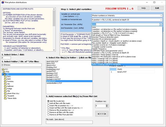
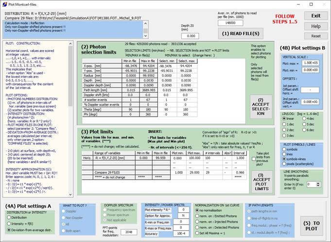
↓Fig. 17. Plot options: choice of axes (“intensity” if vert.axis = none)	↓ Fig.18. Plot options: settings for an intensity plot
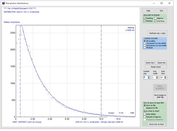
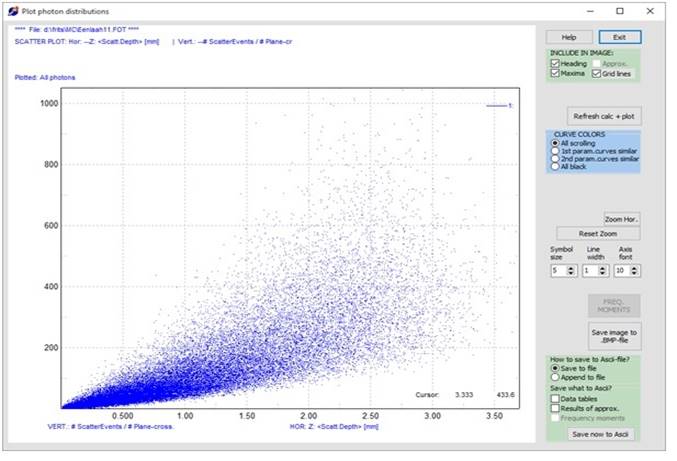
↓ Fig. 19. Intensity plot, with model fitting. Plots of >1 runs optional (with shifts).	↓ Fig. 20. Scatter plot of results. Plots of >1 runs optional (with vert./hor. shifts)
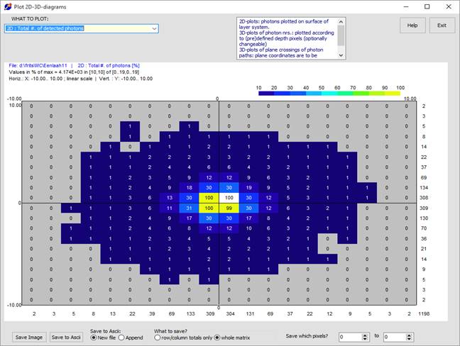
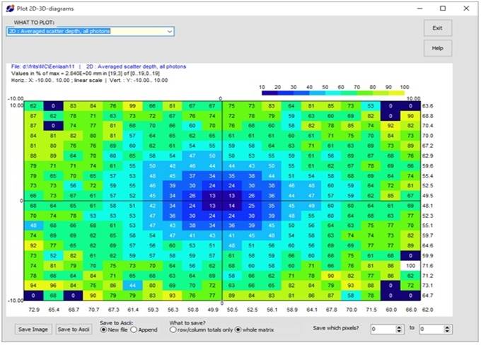
↓ Fig. 21. 2D-plot of results: total number of re-emerging photons.	↓ Fig.22. 2D-plot of results: average scattering depth of all photons.
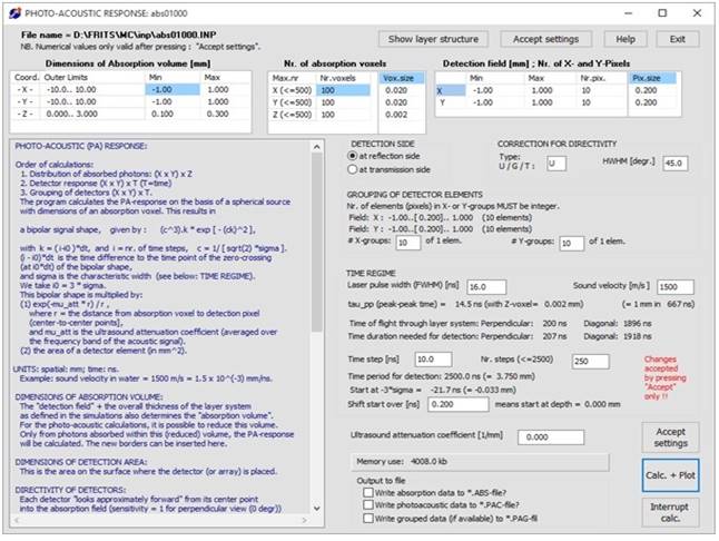
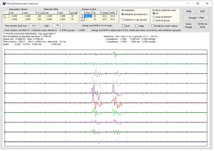
↓ Fig. 23. Photo-acoustic response of absorbed photons: settings	↓ Fig. 24. Photo-acoustic response in 10x10–detector array of 1 tube (Fig.11)
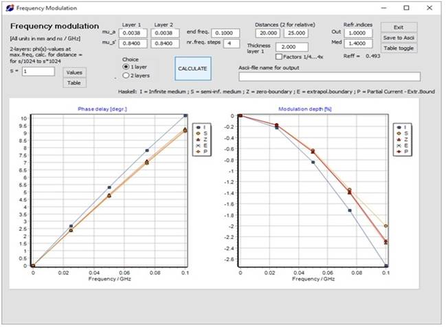
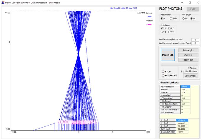
↓ Fig. 25. Extra: frequency modulation of GHz-signals in tissue layers.	↓ Fig. 26. Imaging through a thick convex-concave lens with a few scatterers